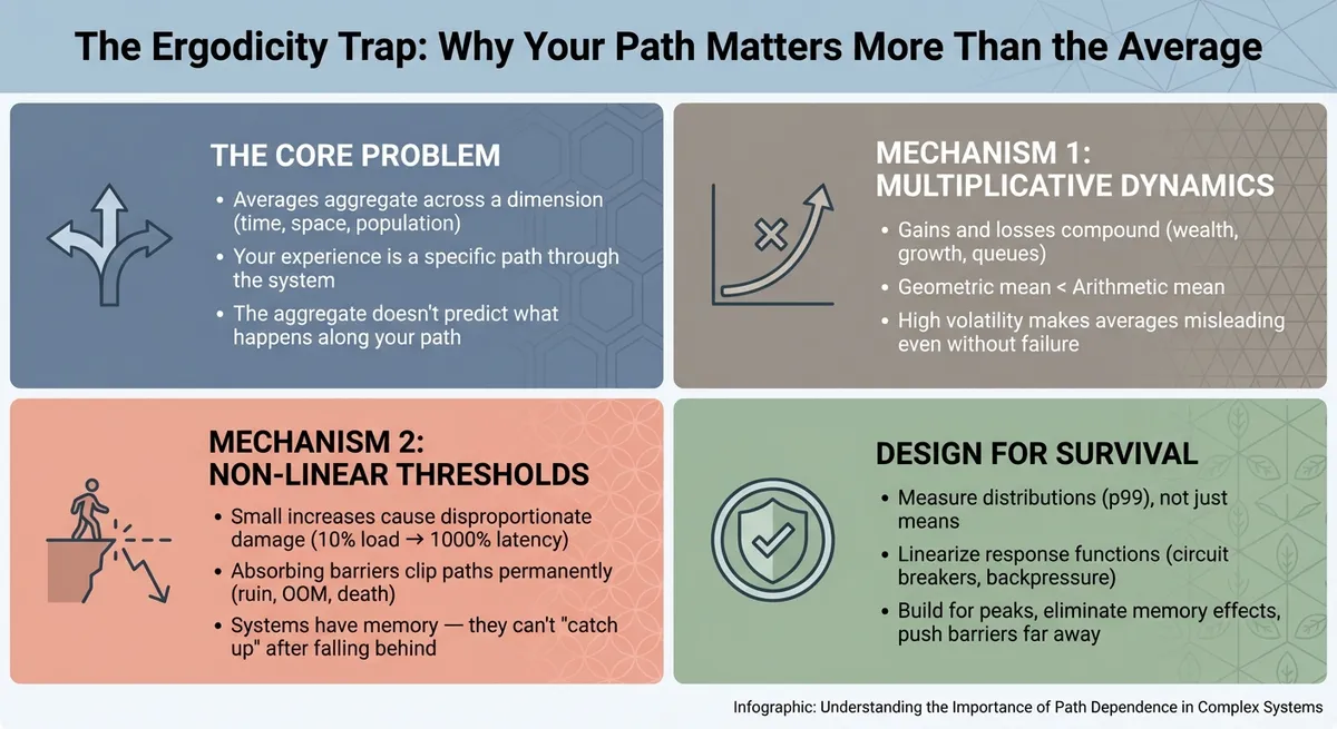
The Ergodicity Trap: Why Your Path Matters More Than the Average

This is a companion piece to my earlier post on Poisson distributions and Prometheus monitoring. There I showed how averages can hide traffic bursts that spike your latency. Here I want to dig deeper into why averages fail—and why the failure isn’t a bug, but a feature of how reality works.

But first, a remark: in that previous post, we got lucky. We survived long enough to diagnose the problem, instrument the fix, and write about it. The bursty traffic degraded our service but didn’t kill it. We’re the survivors telling survivor stories. And that’s exactly what this post is about.

---

There’s an old joke: a statistician drowned crossing a river with an average depth of three feet.¹ The punchline lands because we instinctively know something is wrong with the reasoning—but what exactly?

The statistician’s error wasn’t mathematical. The average was three feet. The error was treating the average as a sufficient summary of the system, ignoring the variance that lurks beneath. The average collapses the shallow shoals and the deep holes into a single, safe number. But the traveler experiences the holes, not the math. At one point, the depth spiked to seven feet, and that extreme value---not the average---determined the outcome.

This is a parable about ergodicity—specifically, about spatial non-ergodicity. The average over space didn’t predict the local experience. And it’s one of the most important and least understood concepts in how we think about systems, risk, and survival.

What Ergodicity Actually Means

The term comes from statistical mechanics, where it has a precise meaning: a system is ergodic if it visits all parts of its state space over time, so that the time-average converges to the ensemble-average. But in recent years, particularly through the work of Ole Peters and the “Ergodicity Economics” program,² the concept has been generalized to ask a broader question: does an aggregate statistic predict what a specific observer experiences along their path?

The classic framing (from physics):

• Ensemble average: Measure a property across many instances of a system at the same moment.
• Time average: Measure a property of one instance across many moments.

If these converge, the system is ergodic. But this conceptual framing—comparing the aggregate to the specific path—extends naturally to other domains:

• Temporal Resolution: Does the average request rate over an hour (the aggregate) predict the load in a specific second (the experience)?
• Spatial Distribution: Does the national hospital occupancy (the aggregate) predict the availability of a bed at your specific local hospital (the experience)?
• Wealth Dynamics: Does the average return across all investors (the ensemble) predict the compounding wealth of one investor over a lifetime (the path)?
• The River Crossing:³ Does the mean depth across the cross-section (the snapshot) predict the safety of the specific sequence of steps taken to cross it (the trajectory)?

In each case, ergodicity is the assumption that the aggregate transfers to the specific path. Non-ergodicity is when it doesn’t—when the journey through the system yields a different result than the snapshot across it.

Most systems we care about—economies, health, infrastructure, servers—are profoundly non-ergodic across at least one of these dimensions.

The Casino Thought Experiment

Nassim Taleb uses a vivid illustration.⁴ Consider two scenarios:

Scenario A: 100 people each go to a casino and gamble once. Some win, some lose. At the end of the day, we count the money. The average return across the group might be, say, -2% (the house edge). But gambler #47 who lost everything has no relationship to gambler #23 who doubled her stake. They’re independent.

Scenario B: One person goes to the casino 100 days in a row. Same game, same odds. What’s their expected outcome?

In Scenario A, the ensemble average works fine. We can predict the casino’s take with confidence. But in Scenario B, something different happens. If there’s any possibility of ruin—going broke—then the time-average diverges from the ensemble-average. The person who goes bust on day 37 doesn’t get to continue playing on day 38. Their personal trajectory terminates.

The ensemble average says “on average, people lose 2%.” But the individual, over time, faces a different reality: eventually, they will hit zero, and the game is over.

This is why the expected value of Russian roulette—a 5/6 chance of winning a million dollars—is mathematically positive (about $833,000) but personally insane. One person playing Russian roulette repeatedly faces eventual certain death, regardless of what the “expected value” says.

Back to the River (and the Server)

In my previous post, I described debugging a service that was breaching SLO despite “normal” traffic. The rate(...[1m]) query showed a comfortable 45 requests per second. But we were dying.

The average was real. The distribution was the problem. Traffic arrived in bursts—180 req/s for a few seconds, then calm. The average smoothed this into a gentle line. But the service didn’t experience the average. It experienced the bursts.

This is the same structure as the river problem. The dashboard was computing an ensemble statistic (what would you expect if you sampled random seconds throughout the hour?), but our service was living through time—and at certain moments in time, it was seven feet underwater.

The ergodic assumption would be: “If the average is 45 req/s, then at any given moment, we’re probably seeing around 45 req/s.” But our traffic was non-ergodic in this sense. The distribution over time wasn’t the same as the distribution at a point. Moments of 20 req/s and moments of 180 req/s averaged to 45, but the service never actually experienced 45.

The Hospital Capacity Problem

Here’s a domain where non-ergodicity manifests across space rather than time: healthcare capacity planning.

A 2025 study published in JAMA Network Open by UCLA researchers reveals a troubling trend.⁵ Post-pandemic, national hospital occupancy has risen from about 64% to 75%. That sounds manageable—plenty of headroom, right?

But 75% average occupancy is dangerously close to failure. Why? Because occupancy isn’t uniform across the territory. It varies by region, by hospital, by department. When a flu wave hits New England while a heat wave stresses Texas, local occupancy can spike to 95% or higher—even though the national average looks fine.

The researchers found that when national ICU occupancy reaches just 75%, there are 12,000 excess deaths in the following two weeks⁶. Not because 75% is inherently catastrophic, but because 75% national means some regions are at 90%+, overwhelmed, turning patients away. States like Rhode Island, Massachusetts, and Washington have already exceeded the 85% threshold that experts consider indicative of a bed shortage.

This is spatial non-ergodicity. The aggregate over space (national average) doesn’t predict the local experience. The average patient has access to a bed. But you are not the average patient. You are a specific person at a specific hospital on a specific night. And the question isn’t “what’s the national occupancy?” but “is there a bed for me, here, now?”

The national average is an ensemble statistic across geography. Your experience is a single point in that space. If you’re unlucky enough to need an ICU bed in Rhode Island during a surge, the comfortable national number provides zero comfort. The aggregate doesn’t transfer to the instance.

Power Grids and Peak Demand

Power grid design faces the same challenge. Average electricity demand is meaningless for reliability planning. What matters is peak demand—and specifically, the shape of that demand over time.

Grid engineers don’t ask “what’s the average load?” They ask “what’s the worst interval we might face, and can we survive it?” They build to peaks, not means. This is explicitly anti-ergodic thinking: acknowledging that the system’s survival depends not on its average state but on its worst-case trajectory.

In South Australia, the 2024 Electricity Report shows that operational demand peaked at 2,748 MW. But crucially, this didn’t happen in the middle of the day. Because of the massive penetration of solar, the grid peak has shifted to 8:00 PM—after the sun has set, but while air conditioners are still blasting.

For 99% of the year, that 2,748 MW capacity looks like “massive overkill.” But in those few critical hours in the evening, the grid either holds or people sit in the dark. The average load tells you nothing about whether the grid survives the sunset.

Why This Matters for Monitoring

Let’s bring this back to software systems. Most dashboards are designed around ergodic assumptions. They show averages, rates, smooth lines. This is fine for steady-state analysis, but it’s actively misleading for failure detection.

Your SLO measures a distribution across moments. When you say “95% of requests complete in under 200ms,” you’re making a statement about specific instances in time. If traffic is bursty, the average request rate can be fine while specific seconds are catastrophic—and those specific seconds are when your users suffer.

The rate(...[1m]) function in Prometheus computes a coarse time-average—it smooths an entire minute into a single number. But your service experiences fine-grained time: each second, each millisecond, sequentially. The “average” second in that minute didn’t exist; there were only quiet seconds and drowning seconds.

This is temporal non-ergodicity: the coarse aggregate over time doesn’t predict what happens at specific moments within that window. The smoothed view and the lived experience diverge.

This is why, in my previous post, the dispersion index mattered. A dispersion index of 1 (variance equals mean) indicates roughly ergodic traffic—the average second looks like any other second, so the aggregate predicts the instance. A ratio of 2.8 signals extreme non-ergodicity: the “average” second doesn’t exist. There are quiet seconds and explosive seconds, and your service has to survive the explosions.

Ensemble-Average Thinking in the Wild

Once you see this pattern, you see it everywhere. The key is identifying: what dimension is being aggregated, and what dimension is being experienced?

Investment returns (aggregate: across time or population → experience: your specific sequence): “The market returns 8% on average” aggregates across years or across investors. But you don’t get the market’s average. You get a specific sequence of returns in a specific order. If you retire in 2008 and need to sell during the crash, the long-run average is cold comfort. Your trajectory diverged from the aggregate.

Career advice (aggregate: across population → experience: your path): “The average software engineer earns $X” aggregates across all engineers. But you’re not sampling from that population—you’re living one path through time, with path-dependent choices that compound or foreclose options.

Drug trials (aggregate: across patients → experience: your response): “On average, this treatment helps” aggregates across the trial population. But it might help 80% of patients enormously and harm 20% catastrophically. If you’re in that 20%, the population average is worse than useless.

Load balancing (aggregate: across servers or requests → experience: one server or request): “Average response time is 50ms” might mean all requests take 50ms (ergodic), or half take 10ms and half take 90ms (non-ergodic). The aggregate masks the bimodal reality that specific users experience.

Why Ergodicity Breaks: Two Distinct Mechanisms

So far I’ve described that ensemble averages diverge from time averages in certain systems. But why does this happen? There are two distinct mechanisms, and conflating them leads to confusion.

Mechanism 1: Multiplicative Dynamics

In a truly ergodic system, every state is recoverable. If you’re down today, you can be up tomorrow. Your trajectory wanders through the state space, and given enough time, it samples all regions in proportion to their probability. Bad luck averages out.

But many real-world processes are multiplicative rather than additive. Your wealth doesn’t grow by adding fixed amounts—it grows (or shrinks) by percentages. Investment returns, business growth, compound interest: all multiplicative.

Here’s why this breaks ergodicity even without any failure or threshold:

Consider the difference between adding and compounding. In an additive process, a loss of $50 and a gain of $50 leaves you unchanged. The fluctuations average out over time. But in a multiplicative process, the order and magnitude matter differently. A 50% loss cuts you in half; to get back to where you started, you don’t need a 50% gain—you need a 100% gain. This asymmetry means that in multiplicative systems, variance inherently reduces your long-term growth rate, creating a gap between the ‘average’ outcome and your personal reality.

In additive dynamics, the arithmetic mean (the simple average) accurately predicts the long run. If you play the game long enough, your total outcome converges to the sum of the averages. But in multiplicative dynamics, the arithmetic mean describes what happens to the ensemble (or parallel universes), not what happens to you over time. For a single trajectory compounding into the future, the relevant metric is the geometric mean. Crucially, the geometric mean is always lower than the arithmetic mean. This mathematical gap—formalized as Jensen’s Inequality⁷ is the ‘volatility tax.’ The more the system fluctuates, the wider the gap becomes, and the more the aggregate average overestimates your actual growth.

This is why high-variance positive-expected-value bets can still be bad for an individual. The ensemble sees the arithmetic mean. The individual experiences the geometric mean. This is why the expected value of Russian roulette—a 5/6 chance of winning a million dollars—is mathematically positive (about $833,000) but personally insane. One person playing Russian roulette repeatedly faces eventual certain death, regardless of what the “expected value” says.

Mechanism 2: Non-Linear Thresholds and Absorbing States

The second mechanism is different: non-linear response functions that create thresholds and absorbing barriers.

Linear systems can absorb fluctuations gracefully—twice the input, twice the output, and you can always reduce back down. But real systems are full of non-linearities:

• Thread pool exhaustion: Below capacity, latency scales gently. At capacity, it explodes. Above capacity, requests start failing.
• Memory pressure: Gradual increase is fine until you hit swap, then performance collapses non-linearly. Hit OOM killer, and processes die.
• Cascade failures: One service times out, causing retries, causing more timeouts. The failure amplifies rather than dampens.
• Queue buildup: Little’s Law (L = λW) describes steady state, but when arrival rate exceeds service rate even briefly, queues grow—and crucially, they don’t automatically shrink back.

This last point deserves emphasis. In an ergodic system, if a server gets “unlucky” and slows down during a burst, it should be able to “catch up” when traffic drops. But queuing dynamics have memory. The requests that piled up during the burst don’t disappear—they still need to be processed. And while you’re draining the queue, new requests keep arriving. If you fell behind far enough, you may never recover.

This is why your server doesn’t need “multiplicative growth” of traffic to be non-ergodic. It has a non-linear cost of processing that traffic. A 10% spike in traffic might cause a 1000% increase in latency. And if the latency increase triggers timeouts, retries, or OOM kills, you’ve hit an absorbing barrier—a state from which recovery is impossible without intervention.

The absorbing barrier at zero (bankruptcy for the gambler, death for the patient, OOM for the server) means that losing trajectories are clipped—removed from the game entirely. The ensemble average still looks fine. Across 100 gamblers, maybe 60 are up and 40 are broke. “Average wealth increased!” But if you’re one of the 40, the average is meaningless. You experienced ruin, not the average.

The Interaction

These mechanisms often combine. Your server might face:

• Multiplicative load growth (traffic that compounds during viral events)
• Non-linear cost curves (latency that explodes at saturation)
• Absorbing barriers (OOM kills, cascade failures)
• Memory effects (queues that don’t drain, connection pools that don’t release)

Each mechanism independently breaks ergodicity. Together, they make the “average” experience a fiction that no specific instance ever lives through.

The Survivorship Problem

There’s a subtle corollary: when we compute ensemble statistics, we often only see the survivors.

The “average startup returns 3x” might be computed only over startups that didn’t die. The “average portfolio return is 8%” might exclude investors who went bankrupt and exited the market. The “average server uptime is 99.9%” might not count the server that failed so hard it was decommissioned.

This survivorship bias makes ensemble statistics even more misleading. The dead trajectories—clipped by absorbing barriers—vanish from the data. What remains looks rosier than reality.

For monitoring, this means: your dashboard showing “average latency” might exclude requests that timed out entirely, or pods that crashed and were replaced, or users who gave up and left. The survivors look fine. But the system, experienced as a trajectory through time, included all those failures.

Designing for Non-Ergodicity

If averages can’t save you, what can? The key is addressing both mechanisms that break ergodicity: multiplicative/compounding dynamics and non-linear thresholds.

1. Linearize your response functions where possible. Circuit breakers, rate limiters, backpressure—these are all techniques for preventing non-linear blowups. If you can turn a cliff into a gentle slope, bursts degrade performance rather than destroying the system. The goal is graceful degradation: twice the load should cause twice the latency, not total failure.

2. Eliminate memory effects that prevent recovery. Queues that don’t drain, connection pools that don’t release, retry storms that amplify—these give your system “memory” that prevents it from recovering when load subsides. Add queue depth limits, implement exponential backoff with jitter, set aggressive timeouts. Let the system forget its bad moments.

3. Push absorbing barriers as far away as possible. What failure modes are terminal? Database corruption, unrecoverable state, cascade failures that bring down the cluster. Build redundancy, enable rollback, design for recovery. You can’t always prevent hitting barriers, but you can make them harder to reach—and recoverable when you do.

4. Measure distributions, not just means. Track percentiles (p50, p95, p99), variance, dispersion. Ask: what does the worst 1% of experience look like? Is it tolerable—or is it an absorbing state? The mean tells you about central tendency. The tail tells you about survival.

5. Build for peaks, not averages. Capacity planning should target peak load, not mean load. Your system needs to survive the hottest second of the busiest day, not the average moment. This is explicitly anti-ergodic design: acknowledging that survival depends on worst-case paths, not expected-case aggregates.

6. Introduce buffers and jitter to convert multiplicative shocks to additive noise. The upstream batch job that crashed our service wasn’t malicious—it just didn’t know it was creating bursts. Adding jitter to batch submissions converted non-ergodic spikes into roughly ergodic flow. Buffers absorb variance; jitter spreads it out. Both reduce the probability of hitting non-linear thresholds.

7. Think in terms of survival probability, not expected value. For any decision with potential ruin, ask: what’s the probability this trajectory survives? A 1% chance of catastrophic failure, repeated daily, is a 97% chance of failure within a year. The expected value might look fine. The survival probability doesn’t.

The Philosophical Residue (and Conclusion)

There’s something philosophically humbling about ergodicity. We love averages because they let us reason about complex systems in simple terms. But averages assume that the statistical properties of the aggregate transfer to specific paths—and they often don’t.

The mechanisms matter: it’s not that averages are “wrong.” It’s that multiplicative dynamics make geometric and arithmetic means diverge, and non-linear thresholds clip specific paths, preventing them from contributing to (or benefiting from) the full distribution. The dead don’t get to average their experience with the living. The bankrupt don’t get to average their returns with the solvent. The crashed server doesn’t get to average its latency with the healthy ones.

You are not a sample from a population. You are a specific path—in a specific place, at a specific time, with a specific history that compounds. The “average human lifespan” is 79 years, but that doesn’t mean you’ll live to 79—and if you encounter an absorbing barrier at 45, no amount of population-averaging helps you.

When Ole Peters reformulated expected utility theory in terms of time-averages rather than ensemble-averages, he found that much “irrational” human behavior—risk aversion, loss aversion, the rejection of positive-expected-value gambles—suddenly looked rational. People aren’t maximizing expectations across hypothetical ensembles; they’re maximizing time-average growth rates for their specific path. What looks like excessive caution from an ensemble perspective is actually optimal behavior for someone who has to live through time and can’t access the parallel universes where their other selves got lucky.

That’s not a bias. That’s wisdom about the structure of the world.

Living the Path

The average exists mathematically but not experientially. You live the path, not the aggregate. So the next time someone reassures you with a dashboard showing a smooth, flat line, don’t ask “what is the average?”

Ask the ergodic questions:

1. What dimension is being aggregated? Are we smoothing over time, space, or population?
2. Are the dynamics additive or multiplicative? Is volatility noise (which cancels out) or a tax (which compounds)?
3. Where are the cliffs? What non-linear thresholds exist where the rules suddenly change?
4. Is there memory? If we fall behind, can we catch up, or does the backlog bury us?
5. Where are the absorbing barriers? What happens to the paths that get clipped—and am I at risk of being one of them?

The statistician drowned because he confused the map (the average) with the territory (the path). Don’t make the same mistake with your systems.

---

Footnotes

1. The drowning statistician has been warning us since at least 1891, according to Quote Investigator—the joke appears in a book about proverbs from Bihar, India, where a clerk ordered his son to ford a stream based on its average depth. The boy drowned. Some lessons never get old. ↩

2. Ole Peters, “The ergodicity problem in economics,” Nature Physics 15 (2019): 1216–1221. This is the canonical reference for a rigorous treatment of ergodicity in economics. ↩

3. A physicist might object that a river isn’t ‘non-ergodic’—it’s just variable in space (heterogeneous). Technically, they are correct. A river is a static object. But the moment you step into the water, you convert that spatial variation into a temporal sequence. ↩

4. Nassim Nicholas Taleb, Skin in the Game: Hidden Asymmetries in Daily Life (New York: Random House, 2018), Chapter 19. ↩

5. Leuchter et al., “Health Care Staffing Shortages and Potential National Hospital Bed Shortage,” JAMA Network Open (2025). ↩

6. Article: US Facing Critical Hospital Bed Shortage ↩

7. Technically, Jensen’s Inequality states that for a concave function (like the logarithm used to calculate compounding), the mean of the function is less than the function of the mean: $\mathbb{E}[\ln(x)] \leq \ln(\mathbb{E}[x])$. In plain English: volatility eats growth. A useful approximation for your realized growth rate is: $\text{Realized Growth} \approx \text{Average Return} - \frac{\text{Variance}}{2}$ If an investment returns +50% one year and -50% the next, the average return is 0%. But the variance is high, so your realized growth is negative ($\approx -13\%$). The dashboard reports the first term (0%); your bank account suffers the second term. ↩